Three-dimensional scaled laboratory experiments, where the deformation is produced in front of you rather than solved for.
Numerical models are only as good as the physics written into them. The laboratory is where that physics is put in the way of a real material: a scaled, three-dimensional experiment deforms under its own buoyancy and viscosity, and the velocity field is measured rather than prescribed. Running the two side by side is what makes a thermo-mechanical model worth believing.
Scale
Three-dimensional, dynamically scaled
Materials
Polydimethylsiloxane, polymer fluids and silicone oils
Measurement
Particle image velocimetry in 2-D and 3-D, with a five-axis robotic arm scanning the surface
Forcing
Density anomaly standing in for eclogite, and thermally dependent convection
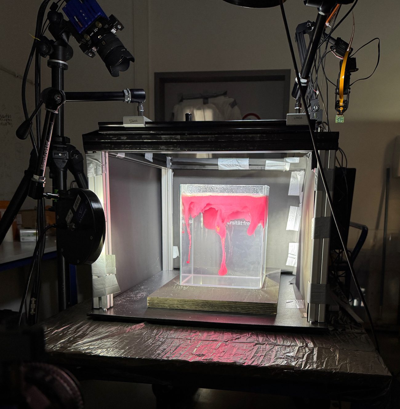
The experimental setup: the tank under its lighting, with the particle image velocimetry cameras and the five-axis robotic surface scanner.
Experiments
Three families of run, separated by what drives them. The first two are density-driven and ask what becomes of a layer too dense to stay where it is; the third is kinematic, and asks how shortening is taken up.
Density-driven
Lithospheric drip
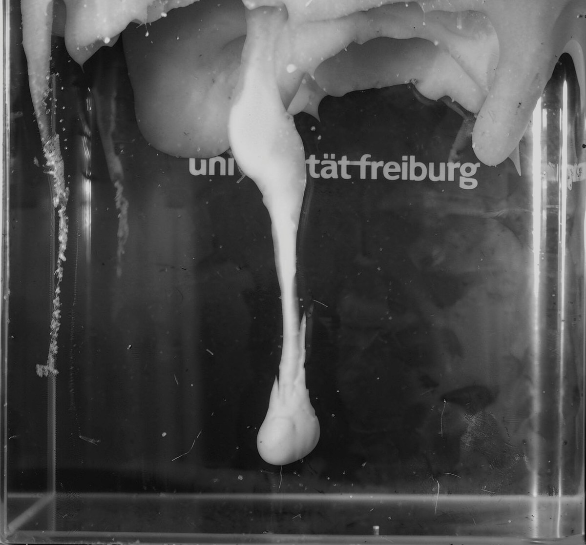
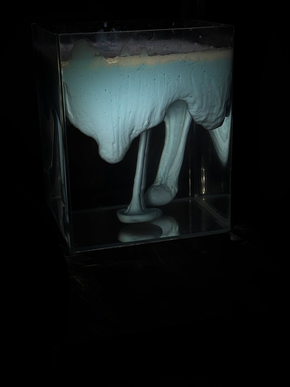
Where the contrast is high the layer pinches into a narrow drip. The run is followed from the first perturbation through necking to detachment, which is the moment that decides whether the dense material is lost to the interior or stays hanging from the layer that made it. A drip is the end member of the instability: nearly all of the dense material gathers into one narrow column, and the layer it came from is left thinned rather than stripped away. The neck is where the outcome is settled, because it is the narrowest part of the flow and therefore the part straining fastest, and it is also the part a two-dimensional section is least able to resolve. Tracer particles seeded through the model make the velocity field readable while all of this is happening, so the growth is measured as it occurs rather than reconstructed afterwards from the shape it leaves behind.
Growth rate and final drip diameter measured against the viscosity contrast across the interface.
Detachment either completes or stalls; both outcomes are recorded, since a stalled drip is its own result.
Surface topography tracked throughout, because uplift and subsidence above the drip is what a planet shows.
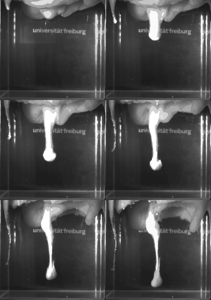
Neck thinning followed frame by frame, since the rate there sets how long the drip has before it either parts or stalls.
Velocity and strain-rate fields recovered by particle image velocimetry during the run, so the growth is measured and not inferred.
A drip descending on a long neck, its head already well clear of the layer that fed it.
A drip at a different viscosity contrast, as a time-lapse: the instability grows, necks and detaches.
Density-driven
Foundering across a layer
Lower the contrast, or let the whole layer go at once, and the behaviour changes: the dense material comes away as a coherent sheet, or as several instabilities competing for the material feeding them. In three dimensions that competition is visible; a cross-section would show one instability and miss it entirely. What separates the two outcomes is how readily the dense layer localises against how fast the fluid beneath it can get out of the way. At a low contrast the layer has no reason to pick a single path, so it descends broadly and keeps its coherence; at a high one the flow gathers into the narrowest route open to it. Between those ends the layer breaks into several drips drawing on a shared reservoir, and the ones that start first starve the ones beside them. The spacing the survivors settle into is the measurement that carries over to a planet, because it is the one a surface can still record long after the layer itself has gone.
Spacing and number of drips measured across the full layer rather than along a single section.
Drips that merge, and drips starved by a neighbour, are both ordinary outcomes here.
The same apparatus covers drip, delamination and coherent foundering: one instability at different viscosity contrasts.
Onset times recorded alongside spacing, because an instability that starts early takes material from the ones next to it.
Each viscosity contrast is tested repeatedly rather than once, and a result is validated by holding it against the earlier repeats; some drips still vary from run to run even when the experimental setup does not.
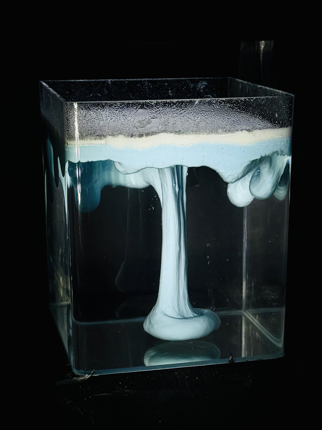
Sheet-like foundering: the dense layer descends as a coherent curtain rather than pinching into a narrow drip. Which of the two happens is set by the viscosity contrast across the interface.
Several instabilities developing across the layer at once, with one already detached and pooled at the base of the tank.
Shortening
Mountain building
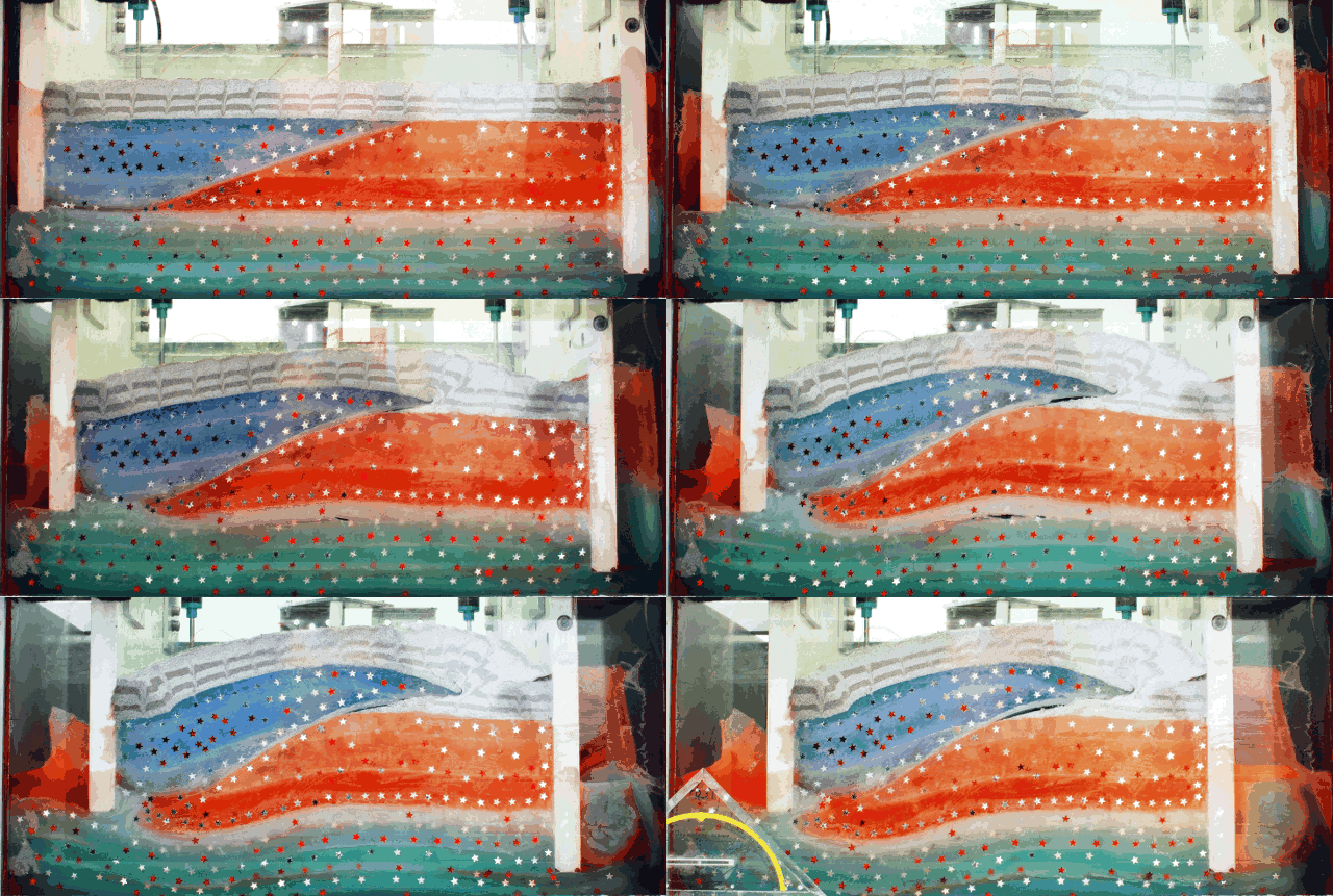
Not every run is density-driven. Layered material put under progressive shortening on the thermo-mechanical deformation apparatus builds a thrust wedge, and the question becomes how that shortening is distributed: which thrusts take it up, in what order they step forward, and what the surface does above them.
Passive markers through the section record the internal deformation, not only the surface expression.
Thrust sequence and spacing read directly off the section as the wedge grows.
Layer strength and thickness varied between runs to change how the wedge partitions the shortening.
Layered analogue material under progressive shortening, building a thrust wedge. The markers scattered through the section record how the deformation is taken up inside it.
Method
How the experiments are built, measured and checked.
Scaling laws
An experiment is only an analogue if the numbers carry. A tank of silicone is centimetres across and runs for an afternoon; the lithosphere it stands for is tens of kilometres thick and takes millions of years, and the two are the same problem only when the dimensionless groups that govern them match. Geometry, density and viscosity are therefore chosen together rather than separately, and the scaling is fixed before a run rather than fitted to it afterwards. What comes out of that is a conversion: a centimetre and an hour in the tank stand for a stated distance and a stated time in the planet, and every measurement quoted from a run is quoted through it.
Length, density and viscosity scales set first; the time and velocity scales follow from them rather than being chosen.
The dimensionless groups matched rather than the quantities themselves: the Rayleigh number for the vigour of convection, the viscosity contrast across the interface, and the ratio of buoyancy to viscous resistance.
Deformation timescale held against thermal diffusion timescale, so a run that is fast enough to watch is not also one that has had time to cool.
Effective viscosities measured for every batch and fed back into the scaling, because a blend that has drifted makes the conversion wrong rather than merely imprecise.
The same scaling carried into the numerical counterpart, which is what allows a laboratory run and a thermo-mechanical model to be compared at all.
Three-dimensional scaled experiments
The experiments are built in three dimensions, not as a cross-section. Lateral escape, along-strike variation and the way a structure terminates are all part of the result, and none of them survive a two-dimensional box. A section cut through a three-dimensional run will often look like a clean two-dimensional experiment, which is exactly the problem: the material that left through the plane of that section is no longer in it to be counted.
Measured in volume rather than in profile, so material that moves out of the plane of a section is still accounted for.
Boundary conditions imposed on a three-dimensional volume: basal drag, lateral confinement and a free upper surface.
Repeat runs across the parameter range rather than a single illustrative experiment.
Materials: polydimethylsiloxane, polymer fluids and silicone oils
The working materials are polydimethylsiloxane, a set of polymer fluids and silicone oils. Polydimethylsiloxane behaves as a very nearly Newtonian fluid at the strain rates these experiments run at, which makes it a dependable stand-in for ductile lithosphere and for the deeper, hotter layers beneath it. Blending it, and layering it against silicone oils of different density and viscosity, builds the stratification a planet actually has.
Viscosity contrast between layers is the control variable: it sets whether a dense layer drips, founders coherently, or simply spreads.
Effective viscosities are measured for every batch rather than taken from a datasheet, because they shift with blend ratio, filler content and temperature.
Density contrasts are tuned with inert fillers, so buoyancy and viscosity can be varied independently.
Starting from a density anomaly
Most of these experiments begin compositionally rather than thermally. A layer is mixed to be denser than the fluid below it, standing in for eclogite: the dense product of a basaltic crust taken through its phase change. Left alone it is unstable, and what follows is the question of whether it drips, founders as a coherent block, or spreads without ever detaching. That outcome is set by the viscosity contrast across the interface and by how fast the dense layer can deform relative to how fast it is loaded.
The density contrast is tuned with inert fillers, so it can be varied without changing the viscosity alongside it.
The same setup covers drip, delamination and foundering: they are the same instability at different viscosity contrasts, not different experiments.
Surface topography is tracked throughout, because the uplift and subsidence above a founding layer is what a planet actually shows us.
Where the process in question is driven by heat, the experiments are run with a thermal boundary condition rather than an imposed velocity. The material's viscosity then depends on its own temperature field, convection organises itself, and the surface deformation is a consequence of that flow instead of something applied at the edge of the box. This is the regime that matters for single-lid planets, where there is no plate boundary to impose motion.
Temperature-dependent viscosity, so the cold upper layer stiffens into a lid exactly as it does on a stagnant-lid planet.
Convection allowed to set its own wavelength and vigour rather than being seeded.
Deformation at the surface read as the product of the interior flow beneath it.
Measuring the flow: particle image velocimetry
The models are seeded with passive tracer particles and imaged through the run, and particle image velocimetry turns those image pairs into a velocity field. That is the point of the method: instead of inferring motion from the final geometry, the full field is recovered while the experiment is still running, which makes strain rate, vorticity and the partitioning of deformation directly measurable.
Surface and internal velocity fields recovered through the experiment, not only at its end.
Strain-rate and vorticity fields derived from the measured velocities, so localisation can be followed as it develops.
The same quantities a numerical model outputs, which is what makes the two directly comparable.
Against the thermo-mechanical models
Each experiment is set up with a numerical counterpart in mind. The laboratory run supplies a measured velocity field under known material properties; the thermo-mechanical model is asked to reproduce it with the same scaled parameters. Where they agree, the numerical rheology is doing its job and can be pushed to planetary conditions the tank cannot reach. Where they disagree, the experiment is usually telling you something is missing from the constitutive law.
Measured effective viscosities and velocity fields used as the benchmark, not a qualitative resemblance of the final shape.
The same scaled parameters driving both, so a mismatch points at the physics rather than at the setup.
Results fed back into the rheology used in MILEVA and MILET.
Lab crew
The experiments are not a one-person job. The lab runs on: